How To Identify Specific Life Forms From Orbit
Why can we detect lianas from space?– biorxiv.org
Lianas, woody vines acting as structural parasites of trees, have profound effects on the composition and structure of tropical forests, impacting tree growth, mortality, and forest succession. Remote sensing offers a powerful tool for quantifying the scale of liana infestation, provided the availability of robust detection methods.
We analyze the consistency and global specificity of spectral signals from liana-infested tree crowns and forest stands, examining the underlying mechanisms. We compiled a database, including leaf reflectance spectra from 5424 leaves, fine-scale airborne reflectance data from 999 liana-infested canopies, and coarse-scale satellite reflectance data covering hectares of liana-infested forest stands. To unravel the mechanisms of the liana spectral signal, we applied mechanistic radiative transfer models across scales, corroborated by field data on liana leaf chemistry and canopy structure.
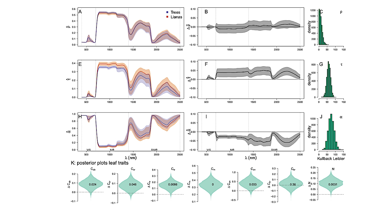
We find a consistent liana spectral signature at canopy and stand scales across sites. This signature mainly arises at the canopy level due to direct effects of leaf angles, resulting in a larger apparent leaf area, and indirect effects from increased light scattering in the NIR and SWIR regions, linked to lianas’ less costly leaf construction compared to trees.
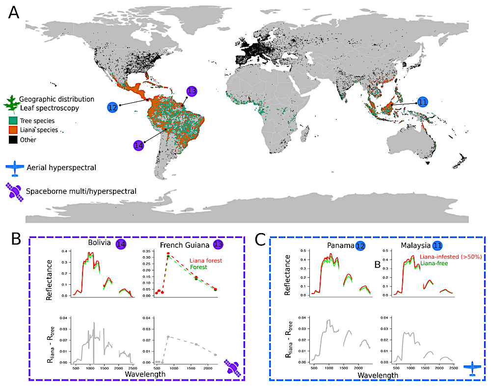
Figure 1. Datasets used in the study to compare the tropical liana and tree spectral signals. Panel A shows the geographic distribution of plants species in the leaf spectroscopy dataset, including the focal tropical liana (orange) and tree species (green). Note that no sampling was conducted in Africa, but three species are common to both the Americas and Africa: Parinari excelsa, Symphonia globulifera and the liana Byttneria catalpifolia. The locations and remote sensing platform types of canopy scale data are given in blue and purple with reference numbers corresponding to Table S1. Panels B and C display liana spectral signals from airborne and spaceborne sensors at focal sites. Top rows show surface reflectance signals of lightly infested forests (Rtree) and heavily-infested forests (Rliana) at each location. Bottom rows show average differences between Rlianas and Rtrees. — biorxiv.org
The existence of a consistent global spectral signal for lianas suggests that large-scale quantification of liana infestation is feasible. However, because the traits identified are not exclusive to lianas, accurate large-scale detection requires rigorously validated remote sensing methods.
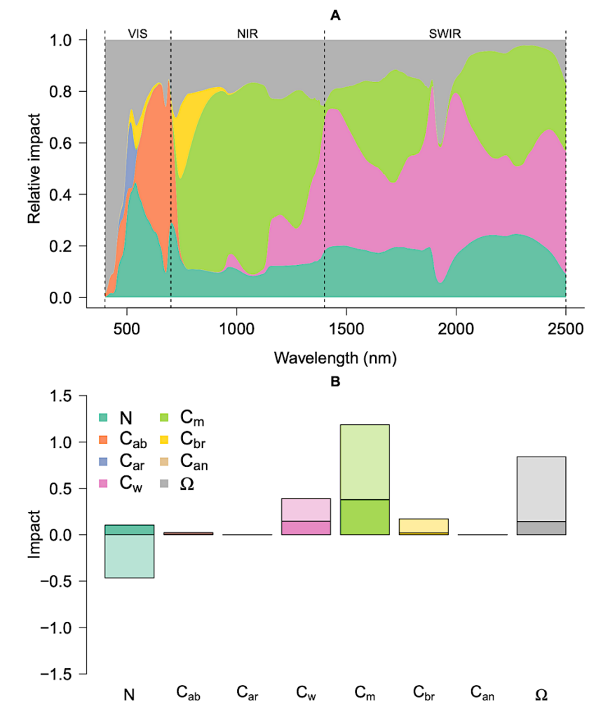
Figure 6. The relative importance of different traits in generating the liana signal across sites.
Here, spectral traits of the top layer were initially set as tree traits and gradually replaced with
liana traits either one by one (additive) or in pairs (interactive effects). The Kullback-Leiber
divergence score was calculated at each iteration. Panel A displays the average relative absolute
impact of changing a single trait in the top layer at each wavelength across all sites. Panel B
shows the total impact of additive (darker colors) and interactive effects (lighter colors). Positive
impact indicates a change towards the liana signal, while negative impact indicates a divergence. — biorxiv.org
Our models highlight challenges in automated detection, such as potential misidentification due to leaf phenology, tree life-history, topography, and climate, especially where the scale of liana infestation is less than a single remote sensing pixel. The observed cross-site patterns also prompt ecological questions about lianas’ adaptive similarities across environments, indicating possible convergent evolution due to shared constraints on leaf biochemical and structural traits.
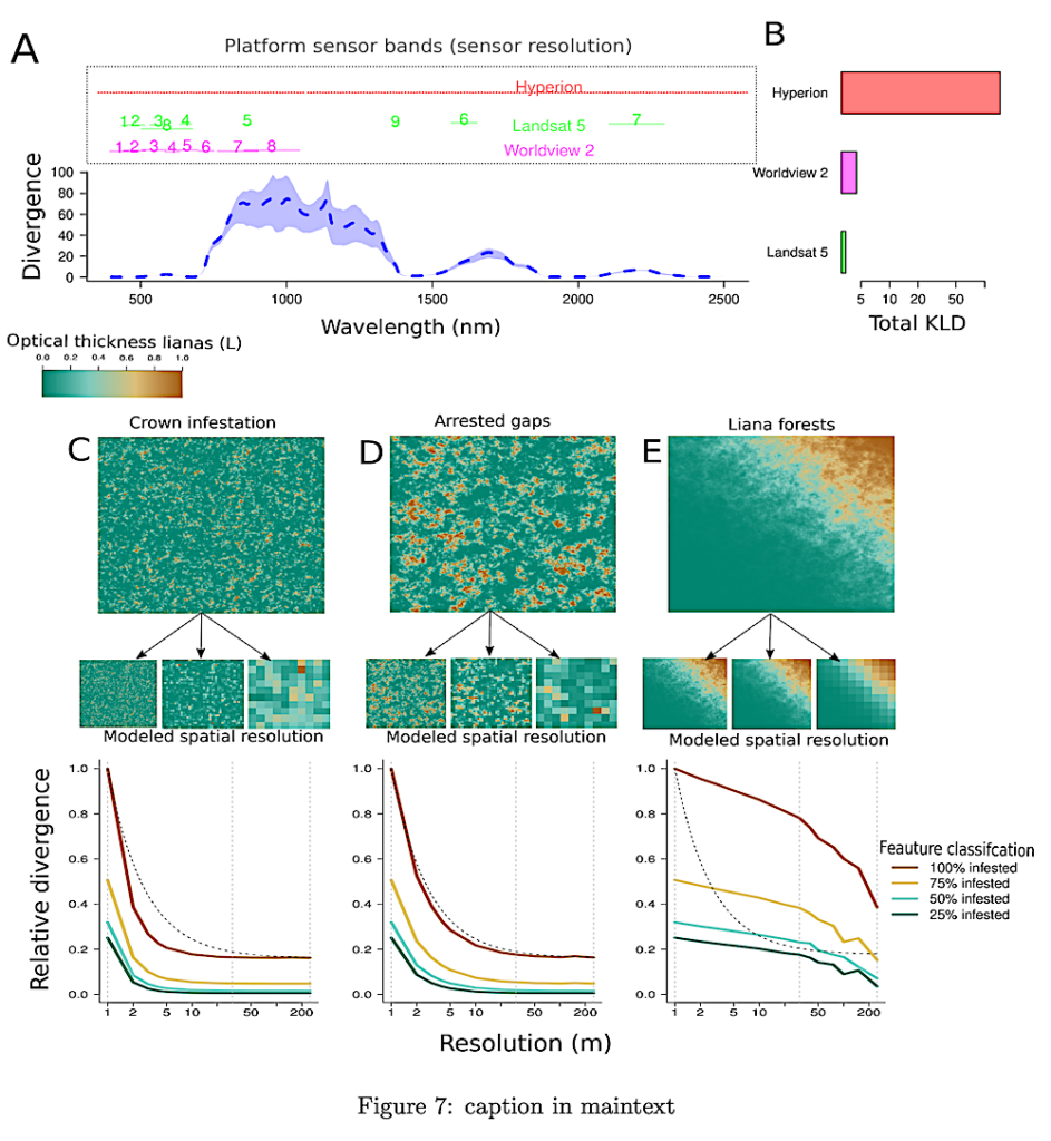
Figure 7. The theoretical capacity of classifiers to distinguish lianas using the expected Kullback-Leiber divergence (KLD). Panel A predicts KLD across wavelengths for 100% liana infestation, with model-based variance estimation, and overlays spectral sampling regions of various remote sensors to assess their effectiveness in liana detection. Panel B presents the cumulative KLD for each sensor, with mean divergences of 0.63 (Hyperion), 0.54 (WorldView 2), and 0.45 (Landsat 5). Panels C-E explore the impact of sensor spatial resolution on liana discernibility at different scales: crown-scale infestation (C), forest gap arrestation (D), and liana forests (E). They include simulated scenes and resampling results, showing the effect on KLD. Liana cluster sizes in these simulations are 350, 2000, and 30,000 m², corresponding to infestation scales from prior studies (Marvin et al. 2016; Chandler et al. 2021; Schnitzer et al., 2000; Foster et al. 2006; Tymen et al. 2016). The colormap indicates liana infestation levels, while line colors in the graphs show different features. Grey vertical lines mark different resolutions, and a black dashed line shows the expected KLD decline for random feature distribution. Each scenario has a roughly equal number of feature pixels. — biorxiv.org
Open data statement Of the 17 datasets used, 10 are published and publicly accessible, with links provided in this submission (Appendix S1: Section S1). Upon acceptance, remaining seven datasets will be provided via Smithsonian’s Dspace. The open-source model code is available as R-package ccrtm (https://cran.r-project.org/web/packages/ccrtm/index.html) and on github (https://github.com/MarcoDVisser/ccrtm). Code will be archived in Zenodo should the manuscript be accepted for publication
Why can we detect lianas from space?
Astrobiology